Synopsis of Trending Scenarios and Impacts of Climate Change on the East African Highlands: The Case of Oromia

Introduction

The source of most of the energy that exists in our atmosphere, including wind, can be traced back to the sun. This energy from the sun is almost constant, and it amounts to ~1368 W/m² before it encounters the earth’s atmosphere where some of the energy is absorbed, and some reflected to space. The reflection and absorption of solar energy depends on several factors such as the season, elevation, and the time of the day. On average only about 70% of the solar constant reaches the earth.

The cause of climate change is, therefore, not the energy that reaches the earth from the sun as it is constant and independent of human activities, but the relatively small amount which humans introduce to the atmosphere in the form of hydrocarbons. In fact, human activities have no capacity to directly change or modify the solar constant. Thus, the malefactor is the energy that is dumped into the atmosphere by human beings, the anthropogenic sources such as oil, natural gas, coal, and nuclear power.

Figure 1.Energy distribution in the atmosphere

Greenhouse gases and their consequences

Gases such as nitrous oxide (N₂O), methane (CH₄), and carbon dioxide (CO₂) are considered greenhouse gases because they trap heat from the sun in the Earth’s atmosphere, leading to a rise in accumulated energy when their concentration increases due to human activities. For example, coincident with CO₂ rise the global average temperature increased by nearly 1^oC. If these trends continue, global temperature could rise significantly leading to disruptive climate change.^[1]

Approximately 50-55% of solar radiation reaching the earth is considered infrared radiation. Infrared radiation is the portion of the electromagnetic radiation emitted by the sun that falls within the infrared wavelength range which typically are from around 780 nanometers (nm) to 1 millimeter (mm) = 1,000,000 nm. This is the thermal component of sunlight that heats an object on earth when absorbed.

Most of the air consists of N₂, (nitrogen, 78%) and O₂, (Oxygen, 21%), and these gases don’t interfere with infrared waves of the sun in the atmosphere. They absorb energy in wavelength range of about 200 nanometers (nm) or less. However, as stated above, infrared energy travels at much wider wavelengths. The ranges that are absorbed by N₂ and O₂ don’t overlap with the infrared range, so N₂ and O₂ don’t intercept infrared waves; the heat waves travel through the atmosphere un-intercepted.

Contrary to N₂ and O₂, greenhouse gases such as CO₂ absorb energy at wavelengths between 2,000 and 15,000 nm. This frequency range overlaps with that of infrared energy frequency, where CO₂ absorbs solar energy at this wavelength. CO₂ absorbs and re-emits the infrared energy back in all directions. About half of the reemitted energy goes out into space, the rest returns to earth as heat. This phenomenon in which absorbed CO₂ energy radiates back to the earth is known as the “greenhouse” effect. Some molecules absorb infrared waves and others don’t. This depends on their geometry and their composition; the number of atoms they are composed of. The natural, pre-industrial CO₂ concentration in the atmosphere kept the energy balance, maintained favorable temperature, and made the earth habitable. Today, a probable runaway level of CO₂ and other greenhouse gases is changing climate as we know it, threatening life on earth.

Source of greenhouse gasses

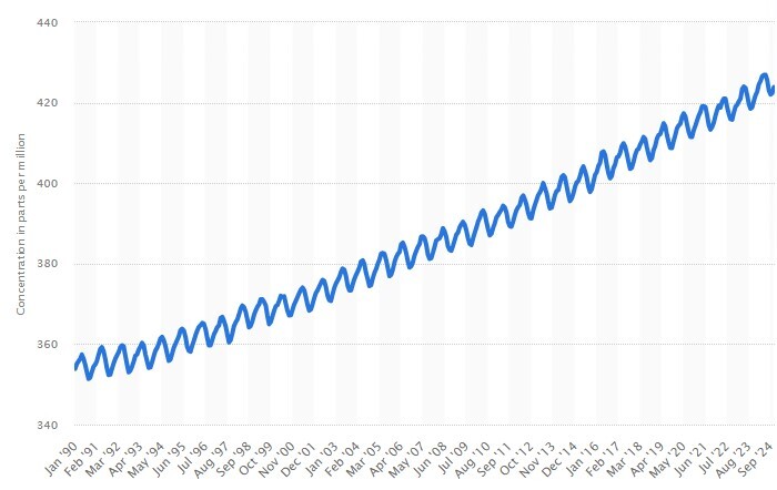
One common byproduct of combustion of hydrocarbons (oil, natural gas, and coal) is CO₂ which is added to the environment. The amount of CO₂ concentration has reached 427 ppm in 2024 from its preindustrial level of 280 ppm, Fig. 2.

Figure 2.The global average concentration of carbon dioxide (CO₂) in the atmosphere, Source: globalchange.gov^[2]

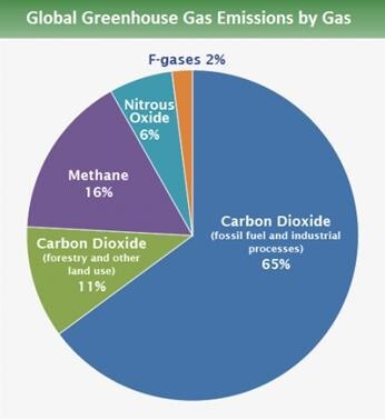
Volume wise, CO₂ constitutes the largest global greenhouse gas emission. CH₄ and N₂O come far behind (Fig. 3). However, the energy absorbing intensity, the climate change potential of N₂O is much greater than that of CO₂ and CH₄. Taking the greenhouse effect of CO₂ as a reference point, CH₄ and N2O have 21- and 310-times global climate change potentials, respectively, Beyene and Zevenhoven.^[3] High temperature combustion is the main source of N₂O, whereas composting, oil and gas extractions are to blame for most of the CH₄.

Figure 3.Emissions by gas typeSource: IPCC (2014) based on global emissions from 2010.

Quantifying the sources

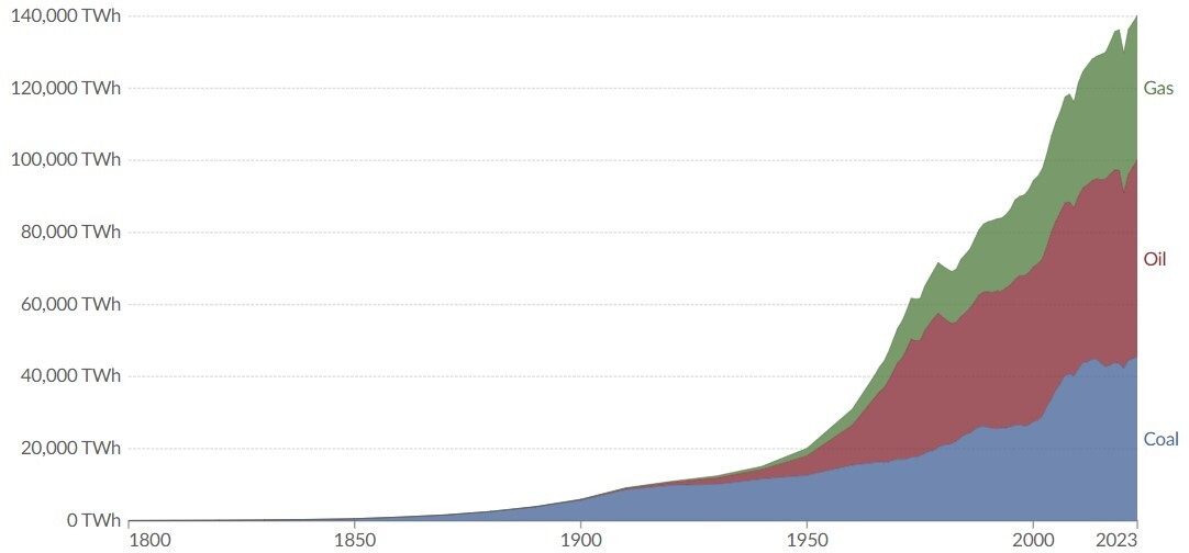
Since the excavated amount of these resources is known globally, and since they carry a known amount of energy per mass, the anthropogenic heat dumped to the atmosphere can be estimated somewhat accurately using, for example, the peak extraction method. The combined sum of energy at peak for oil, natural gas, and coal, Fig. 4, is about 4.15409E+14 MJ/yr.^[4] This estimate excludes the 440 or so commercial nuclear power reactors operating in about 30 countries with about 377 GW of total capacity. These reactors add about 15% to the global electric supply, therefore, about that much to the control volume. There are also about 180 nuclear reactors powering some 140 ships and submarines of primarily military applications. The latter, nuclear reactors are neglected in this analysis.

Figure 4.Global fossil fuel consumption, Source: ourworldindata.org^[5]

Specific humidity can be used to further explain the impact of this anthropogenic heat on climate. Assuming 25°C dry bulb temperature, relative humidity of 40%, specific humidity of 8g/kg, for a generally accepted atmospheric air mass 5.15×10¹⁸ kg, the total kg of vapor in the atmosphere would be 4.12×10¹⁶ kg. The impact of this mass of vapor on pressure gradients and wind velocity are a subject of momentum and continuity equations.

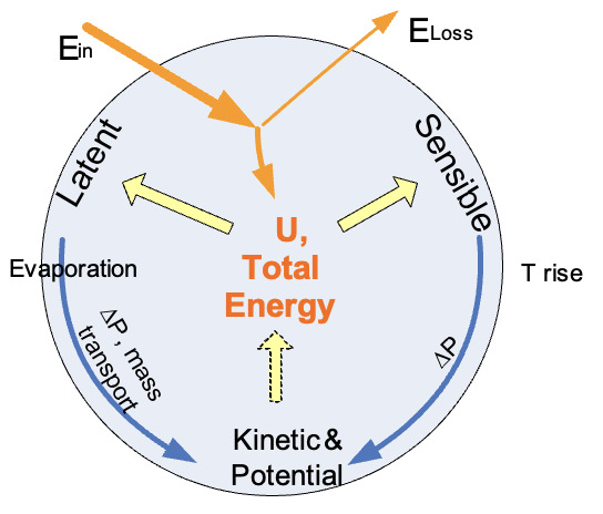
The energy in the atmosphere is spent in two ways: sensible heat and latent heat. Sensible heat is the energy that changes the temperature of a substance without changing its phase. Latent heat is the energy that causes phase change without increasing the temperature.

To better understand the impact of latent heat, we conveniently introduce the concept of “Equivalent Rate of Evaporation”, (ERE) defined as the total amount of moisture that could be added to the atmosphere if the entire Q_E were taken as H_L. This hypothetical scenario helps quantify the extreme scenario as an asymptote. For known enthalpy of vaporization, 2257 kJ/kg = 2.257MJ/kg, the annual ERE for 25 billion barrels/yr of oil alone would be 6.77816E+13 liter of water/yr. Assuming all the heat is latent, this much water would be added to the atmosphere because of combustion of oil.

Based on this approach, it was determined that the total of energy at peak for oil, natural gas, and coal is about 4.15409×10¹⁴ MJ/yr, which is equivalent to the energy needed to evaporate 1.7 times the annual flow of the river Nile.^[6] For example, assuming 25°C dry bulb temperature, and relative humidity of 40%, with specific humidity of 8g/kg, this energy would translate into ERE of about 0.447% for the yr. One may see this as a small percentage of natural solar energy. However, the impact of this added energy is further intensified by “secondary effects,” indirect or induced changes that happen because of a primary action occurring later in time at the same place or at a distant place.

Secondary Effects

Secondary effects cause ripple upshots which are added to the primary environmental impact, and the consequences can be larger than the primary effects.

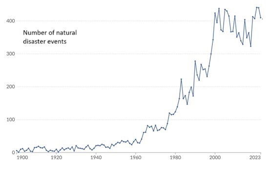
For example, as evaporation increases, a secondary effect of increased moisture in the atmosphere induces more intense, frequent, heavy rainfall, flooding, and stronger hurricanes. Warmer air holds more moisture, leading to heavier precipitation when storms form. Secondary effects can change mosquito habitat and favor growth of mosquitoes with the spread of diseases like malaria in areas not known before. Economic and political instabilities from climate-related disasters, resource scarcity, increased air pollution, and more frequent wildfires can result from climate change as secondary effects, Fig. 5.

Figure 5.A century of weather-related disasters, Source: OurWorldinData^[7]

Impact of Climate Change on East Africa and Oromia

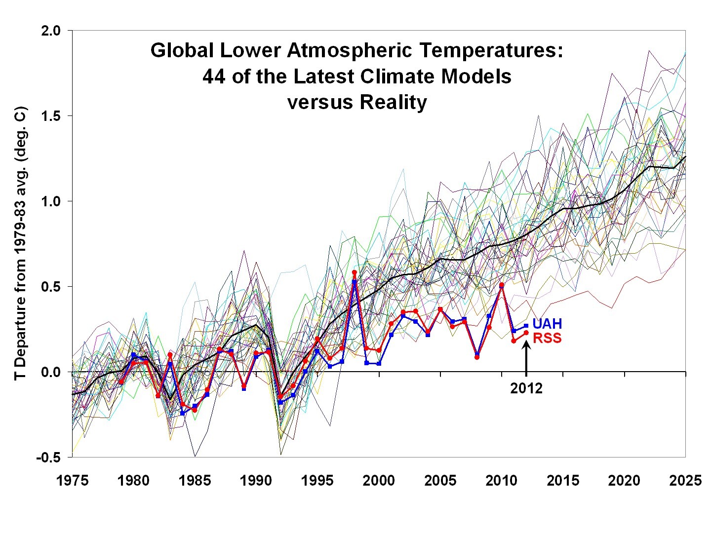
Single climate models can be inaccurate and unreliable, hence should not be taken seriously. However, there are ways to evaluate the accuracy of models. Two ways of measuring the accuracy of predicting climate change is by comparing consistency of the results among the models, as well as agreement of the models with observations both temporally and spatially, Fig. 6.

Figure 6.Temperature changes relative to the 1979 to 1983 average as predicted by 44 climate models. Source: https://www.drroyspencer.com/2013/04/global-warming-slowdown-the-view-from-space/, republished with permission.

Figure 6 shows thin colored lines and two satellite-derived estimates, labeled as UAH and RSS. The bold black line is the average temperature change for all the 44 models. This average is used in the IPCC reports. One major conclusion that follows the trend of the lines in Fig. 6 is that all the models agree there will be a temperature increase despite disagreements on just by how much.

The average annual precipitation or temperature projections by singular climate models should be approached cautiously because the predicted changes may mask vivid inaccuracies. As an example of model consistency, we can take the decadal trend (Fig. 7) showcasing four scenarios of observations for years from 1951 to 2003: cold nights, cold days, warm nights, and warm days. These model trends show no change in the east African highlands over the cited period.^[8] Thus, the daily extreme temperatures in east Africa remain unimpacted which is not the case for most parts of the world. While many climate models and predictions agree very well on some forecasts, there can be sharp disagreements in many cases.

Figure 7.Annual average change in precipitation between today and the end of the century, dots indicate areas where at least nine out of 10 models agree on the direction of change. Source: carbonbrief.org; adopted from European Climate Assessment & Dataset project^[9]

Figure 7 demonstrates another case where models agree or disagree on how average precipitation will change in the future. The dots in the figure indicate areas where at least nine out of 10 models agree on the direction of such change. The East African highlands are areas where many models agree regarding the annual average change in precipitation between today and the end of the century.

Recapping the theme of the subtopic, there are model agreements on the current climate change projections for the East African Highlands, which are expected to see increased rainfall. The studies indicate a potential rise in precipitation amounts across the region including in the highlands of Oromia, which overlaps the central and northern parts of Ethiopia.^[10]

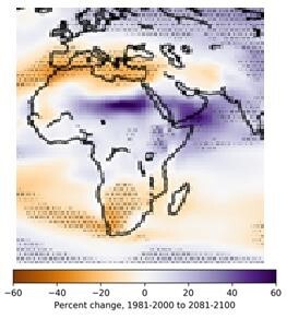
Figure 9 shows that the Ethiopian highlands will exhibit increased rainfall while drought increases in most other parts of Africa. Unfortunately, the predicted increase in precipitation comes with variability in rainfall patterns within the highlands which must be a significant concern.^[11]

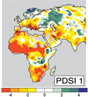
Figure 8 shows the relative dryness of a region using the Palmer Drought Severity Index (PDSI) index. PDSI is used to estimate the severity and duration of droughts. It measures the cumulative deficit (relative to local mean conditions) in surface land moisture by incorporating precipitation data between 1900 and 2002, into a hydrological accounting system. Red and orange areas are drier (wetter) than average and blue and green areas are wetter (drier). It confirms a widespread increase of drought in Africa, except the East African Highlands and central Africa.

Data and climate models consistently show that autumn, summer, and spring in East African highlands will exhibit little or no change in climate. The major change is in the winter which exhibits increased rainfall. The increased rate of precipitation in the highlands within the same rainy season suggests that the rain comes with increased intensity, carrying secondary effects of increased erosion, flood, and landslides.^[12]

Figure 8.Changes in precipitation for distribution of mean precipitation changes at small regional scales, i.e., within the highlands,^[13] 1900 to 2002. East Africa sees increases despite agreement of climate model studies regarding in rainfall and cloud counter increased intensity and decreased frequency in the warming. Source: IPCC^[14]

In addition to the increased rate of precipitation within the same short rainy season - resulting in increased intensity there is also unpredictability in small scale temporal and spatial distribution of the rain. The climate models show poor consistency on predictions of distribution of mean precipitation changes, particularly at a regional scale, i.e., within the highlands,^[15] despite agreement of climate model studies regarding increased intensity and decreased frequency in the highlands to accompany climate change which is thoroughly discussed in the literature.^[16] Although accuracy of predicting regional (small area) precipitation distribution is far from acceptable, evidence for the prevalence of “increased intensity and decreased frequency” is well-reported, Trenberth et al.^[17] Chou et al write that the increase in rainfall in East Africa, extending into the Horn of Africa, is robust across the ensemble of models, with 18 of 21 models projecting an increase in the core of this region. However, the increase in the average doesn’t predict consistency in time.^[18]

In the tropics, a weakening circulation does compensate for the effects of increased atmospheric moisture. Models foresee a widening of the seasonal precipitation range between wet and dry seasons. For large spatial averages, the amplitude for the increase and decrease of precipitation agrees relatively well among climate models, with some discrepancy in identifying the locations of the peak predictions.

“Upped-ante” vs “rich-get-richer” mechanism, impact on highlands

As tropical troposphere warms, say because of El Niño or increased greenhouse gas effect, the atmospheric boundary layer (near the surface of the earth) will have increased convection.^[19] The increased convection is balanced as added horizontal energy transfer from adjacent moisture source. This extra moisture transport is too high a draw from the adjacent zone and could lead to drought conditions at certain convective margins, known as the “upped ante” mechanism, Fig. 9. This mechanism for increased precipitation near the centers of convective zones is known as the “rich-get-richer” mechanism. Based on this scenario, in its simplified form the atmospheric moisture will tend to increase in warmer climate, which suggests higher precipitation in tropical convergence zones.^[20]

Figure 9.Upped-ante mechanism

In a simplified context, the “wet-gets-wetter” mechanism predicts that rainfall should increase in regions that already have much rain, leaving a tendency for dry regions to get dryer, Fig. 9. The “warmer-gets-wetter” mechanism on the other hand predicts rainfall should increase in regions where sea surface temperature rises above the tropical average warming.

It seems that dynamic feedback via changes in vertical velocity are key to the precipitation anomalies associated with both the upped-ante and rich-get-richer mechanisms over the tropics. These dynamical convergence feedback can enhance or decrease the magnitude of the precipitation anomaly. The spatially inhomogeneous occurrence suggests the theory and the model elements are still grossly imperfect.

The upped-ante mechanism, while making the highlands of Oromia wetter, could make the lowlands such as the Borana region dryer.

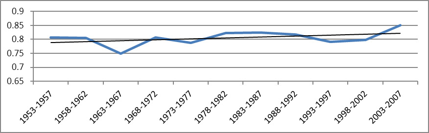
Shift: Based on climate data and simulations, a recently published paper discusses significant shifts in rainfall patterns around the Amazon, sub-Saharan Africa or East Asia, with a tendency to shift tropical rainfall northward. As such, the authors suggest that the inter-hemispheric temperature be taken as a relevant indicator of hemispheric and perhaps regional climate change. This temperature gradient is likely to impart terrestrial shift of seasons, causing shifts of the wet season from south to north in Africa and South America. The leading drive of this shift is probably uneven warming of the Earth, i.e., the Northern Hemisphere contains more land mass, and hence it warms faster than the ocean-dominated south. The hemispherical temperature difference will in turn drive changes in tropical rainfall which respond more to the temperature difference between the two hemispheres.

This shift in rain bands northward because of sudden changes in the temperature differential are irritants to weather patterns on the equatorial tropics. The one-half Fahrenheit degree change that occurred in the late 1960s coincided with a 30-year drought in sub-Saharan African, with far reaching consequences to livelihood and the economy including famine, – with changes on climate signature, with increased desertification across North Africa. This temperature anomaly also corresponded to a decrease in the monsoon activity across East Asia and India. The paper also makes some important conclusions, supporting the wet-gets-wetter mechanism. But the authors also found evidence for the “warmer-gets-wetter” mechanism, i.e. higher surface temperature induces increased rainfall. Thus, the study shows that the two mechanisms are complementary near the Equator because the warming ocean induces more convection rainfall, whereas the rising temperature causes drier pattern further away from the Equator, making the warmer get wetter. As this band of increased rain oscillates across the Equator with the Sun, it causes seasonal rainfall anomalies that follow the wet-gets-wetter scenario, which contributes more to seasonal rainfall changes, whereas the warmer-gets-warmer is paired more with mean annual rainfall changes.

The predicted north-ward shift will be overshadowed by the increased precipitation in the highlands and the upped-ante in the region, hence, may not have a pronounced impact on East Africa.

Regional Precipitation data

Over the last several decades several countries have constituted a data gathering system for relevant climatic coordinates such as temperature and rainfall. The data carry a wealth of information to assess trends, although even the several decades of data gathering remains short compared to the lifespan of atmospheric cycles and changes. The data also does not distinguish changes because of natural phenomenon from those caused by human intervention. Despite these flaws, the numbers, even on a short-term scale, offer interesting conclusions that cannot be ignored as natural or reversible trends.

The nine sites have diverse latitude, altitude, as well as elevation – with traditional precipitation rate ranging from low to high. The data cover at least 50 years of monthly precipitation records.

The data are sanitized where obvious intervention was needed, and a process of trend analysis is designed as below.

Data preparation

I. We determine the monthly mean precipitation of each month for a span of five years. Let that be equal to X_n. For example, the mean of all January precipitations for the first five consecutive years of case 1, X₁ =30.40mm

II. We calculate the annual sum of precipitation for each of the five years, and then take the average of the sums of all the five years as R. For case 1, as an example, R = 1089.34

III. We divide the R value by twelve and subtract it from the monthly mean precipitation, Xn for all the twelve months and register their absolute values Rx as the seasonal index. Thus,$\left| R_{x} = \ X_{n} - \frac{R}{12} \right|$ and for case 1, R₁ = 60.38.

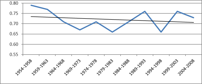
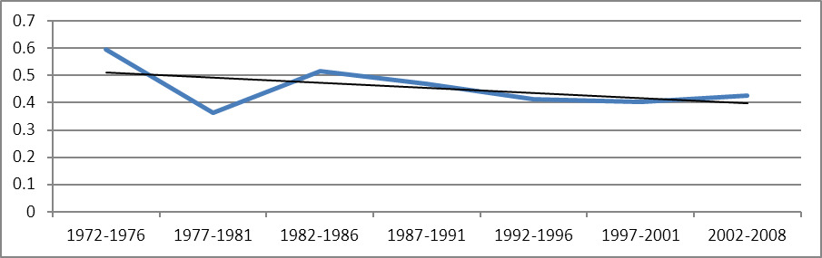
IV. We take the sum of R_x and divide it by R to get scatter trend coefficient, ST, (Eq. 1), which for the case we have followed above is equal to 0.79, as shown below. The remaining values of ST are given in Tab. 3. Thus,

$$ST = \ \frac{1}{R}\sum_{n = 1}^{12}\left| X_{n} - \frac{R}{12} \right|\tag{1}$$

For example,

ST = (1/1089.34)*[(30.40-(1089.34/12))+(41.64-(1089.34/12))+(45.96-(1089.34/12))+(60.88-(1089.34/12))+(60.70-(1089.34/12))+……….+(3.80-(1089.34/12))] = 0.79.

Using the same procedure outlined above, the mean of all January precipitations for the first five consecutive years of two sites, we get Fig. 10 through Fig. 12.

Figure 10.Seasonal scatter slope based on 5–year averages of the trend coefficient for Case 1, Finfinnee, showing downward slope of 0.0028.

Figure 11.Seasonal scatter slope based on 5 –year averages of the trend coefficient for Case 2, downward slope of 0.0188

Figure 12.Seasonal scatter slope based on 5 –year averages of the trend coefficient for Case 3, upward curve with a slope of 0.0033.

Conclusion

Climate models show that there will be increased precipitation in the East African highlands, but spanning in the same rainy season, accompanied by unpredictability, high in intensity. More rain in the same duration would mean flooding, landslides, and other secondary effects are expected. The upped-ante mechanism, while making the highlands of the region wetter, could render the lowlands such as the Borana region even dryer. The predicted north-ward shift will be overshadowed by the increased precipitation in the highlands and the upped-ante in the region, hence, may not have a pronounced impact on East Africa.

Two of the 9 cases examined here show significant slope in the scatter trend, which demonstrates that the rainy season is shifting to either earlier period or later times in the annual cycle. The difference between the maximum and minimum of the five-year averages for the 50 or so years, combined with the slopes shown, the figures show what has been observed over the last few decades, that farmers have more and more difficulty predicting the beginning of the rainy season.

The following solutions can be envisioned as climate mitigation measures:

a. The necessary move towards climate mitigation in Oromia and Ethiopia must be converting agriculture from rain-dependent to irrigation dependent. This is critical to the country especially when other aggravating reasons such as rapid population increase are considered. Irrigation need not be large dams. Dams that are less than 5 meters high providing an impoundment of 100 surface acres or less can go a long way towards making farming independent of the rain.

b. Extensive water storage system. This provides opportunities for multi-cropping where farmers plant two or more crops successively on the same field within a single year. In Southern California, a significant portion of agricultural land is used for irrigation, with roughly 8.5 million acres of land being irrigated, representing about one-fifth of all working lands in the state.

c. Reforestation and forest protection - to restore lost forests and reset the balance in the critical ecosystems. Forests absorb CO₂, filter pollutants and chemicals from water, making it safer for human use, and prevent erosion enriching the soil with organic matter.

d. Energy supply to towns and large villages is essential to curb down dependency on charcoal. Charcoal as a major fuel source has depleted the country of its valuable forests thereby leaving wildlife without shelters. Investing in renewable energy sources like wind, solar, and hydropower is important to reforest the country.

e. Transportation is important for any development. However, to grow without pollution, it is important to expand electric-driven transportation systems.

f. Climate technologies, i.e., using drought-resistant crops, installing early warning systems to predict El Nino should be considered a priority.